Linear Regression
Published:
![]()
MindNotes - Deep Learning - Linear Regression
Author: Christian M.M. Frey
E-Mail: christianmaxmike@gmail.com
PyTorch - Linear Regression
In this tutorial we have to solve basic tasks in pytorch and also a linear regression problem using both, an analytical solution as well as iteratively learning a linear regression model. It is recommended to look up the basic learning procedure in pytorch and how the forward methods for learning a model can be used. Let’s code!
Load dependencies
import torch
import torch.autograd as autograd
import matplotlib.pyplot as plt
import numpy as np
torch.__version__
'1.9.0'
1. Recap: Basics
a) Create a tensor of shape (2, 5, 5) with random numbers from a standard normal distribution! Print the shape!
t = torch.randn(2,5,5)

print(t.size())
torch.Size([2, 5, 5])
b) Create a tensor with floats from the following matrix
M = [[1, 2, 3], [4, 5, 6]]
M_tensor = torch.FloatTensor(M)
print(M_tensor)
tensor([[1., 2., 3.],
        [4., 5., 6.]])
c) Get the 2nd column and the 1st row of the tensor matrix created in b) respectively
print(M_tensor[:, 1])
print(M_tensor[0, :])
tensor([2., 5.])
tensor([1., 2., 3.])
d) Reshape the following tensor to become two dimensional with shape = (9, 3) and get the mean per column
x = torch.randn(3, 3, 3)
print(x)
tensor([[[ 2.1519,  1.4420, -0.2922],
         [ 0.7861, -0.2995, -0.2915],
         [-1.9797, -0.4868,  0.4467]],

        [[-0.9134, -0.9735,  0.8034],
         [ 0.8848, -0.5493, -1.3184],
         [-0.7388, -2.3136,  1.0428]],

        [[-0.4044,  0.7170, -0.6831],
         [ 1.9426, -0.1602, -1.6435],
         [ 0.2225,  0.2656,  0.2089]]])
x_reshaped = x.view(9, 3)
print(x_reshaped)
print(x_reshaped.mean(dim=0))
tensor([[ 2.1519,  1.4420, -0.2922],
        [ 0.7861, -0.2995, -0.2915],
        [-1.9797, -0.4868,  0.4467],
        [-0.9134, -0.9735,  0.8034],
        [ 0.8848, -0.5493, -1.3184],
        [-0.7388, -2.3136,  1.0428],
        [-0.4044,  0.7170, -0.6831],
        [ 1.9426, -0.1602, -1.6435],
        [ 0.2225,  0.2656,  0.2089]])
tensor([ 0.2169, -0.2620, -0.1919])
e) Convert the following tensor into a numpy tensor
t = torch.ones(10)
print(t)
tensor([1., 1., 1., 1., 1., 1., 1., 1., 1., 1.])
n = t.numpy()
print(n)
[1. 1. 1. 1. 1. 1. 1. 1. 1. 1.]
2. Gradients with PyTorch
In the following cell, get the gradients of s with respect to x and y respectively. Play around with other functions/gradients
#calculate gradients
x = torch.tensor([1., 2., 3.]).requires_grad_()
y = torch.tensor([4., 5., 6.]).requires_grad_()
z = 2*x + y**2
s = z.sum()
print(z.grad_fn)
print(s.grad_fn)
<AddBackward0 object at 0x7fae06da5400>
<SumBackward0 object at 0x7fae06da59e8>
s.backward()
print("ds/dx\n", x.grad)
print("ds/dy\n", y.grad)

#Be careful: by default, gradients accumulate everytime you call them! Thus, call:
x.grad.zero_()
y.grad.zero_()
ds/dx
 tensor([2., 2., 2.])
ds/dy
 tensor([ 8., 10., 12.])


tensor([0., 0., 0.])
3. Simple Linear Regression
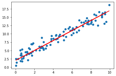
a) Solve the following linear regression problem analytically. Compare the result for different values of n!
torch.manual_seed(3)

n = 100
d = 1
x = torch.FloatTensor(n, d).uniform_(0, 10)
noise = torch.FloatTensor(n, d).normal_(0, 1)

t = 2    #intercept
m = 1.5  #slope


y = m*x + t + noise
r = m*x + t #regression line, just for plotting

plt.scatter(x, y)
plt.plot(x.numpy(), r.numpy(), 'r')
plt.show()
m_pred = ((x - x.mean()) * (y - y.mean())).sum()/ ((x - x.mean())**2).sum() #slope
t_pred = y.mean() - m* x.mean() #intercept
print("Y = {:.2f}*x + {:.2f}".format(m_pred, t_pred))
Y = 1.43*x + 2.11
b) Fill in the missing parts of the LinearRegression model below.
The forward method should just return a linear function of x.
Train the model to learn the parameters above!
See what happens for different learning rates!
import torch.nn as nn
import math
#calculate minimal possible MSE loss
y_perfect = m*x + t #without noise
nn.MSELoss()(y, y_perfect)  # => as threshold for training
tensor(1.2995)
class LinearRegression(nn.Module):

    def __init__(self, in_dim, out_dim):

        super(LinearRegression, self).__init__()
        # Calling Super Class's constructor
        self.linear = nn.Linear(in_dim, out_dim)

    def forward(self, x):
        out = self.linear(x)  # Here the forward pass is simply a linear function
        return out

IN_DIM = 1
OUT_DIM = 1

#1. Create instance of model
model = LinearRegression(IN_DIM, OUT_DIM)

#2. Define Loss
loss_function = nn.MSELoss() # Mean Squared Error

#3. Setup Training
alpha = 0.02 #learning rate
optimizer = torch.optim.SGD(model.parameters(), lr=alpha)

#4. Train the model
MAX_EPOCHS = 500
THRESHOLD = 1.3

for epoch in range(MAX_EPOCHS):
    optimizer.zero_grad() #clear gradients
    y_pred = model(x)  #run model.forward() to get our prediction
    loss = loss_function(y_pred, y)
    loss.backward()     #back propagation
    optimizer.step()    #update parameters
    if epoch%10==0:
        print('epoch {}, loss {}'.format(epoch,loss.data))
    if loss.data < 1.3:
        break;
epoch 0, loss 90.17665100097656
epoch 10, loss 2.5911574363708496
epoch 20, loss 2.3015341758728027
epoch 30, loss 2.0744073390960693
epoch 40, loss 1.8962912559509277
epoch 50, loss 1.7566097974777222
epoch 60, loss 1.647068977355957
epoch 70, loss 1.5611660480499268
epoch 80, loss 1.4937993288040161
epoch 90, loss 1.4409695863723755
epoch 100, loss 1.3995394706726074
epoch 110, loss 1.3670496940612793
epoch 120, loss 1.3415703773498535
epoch 130, loss 1.3215889930725098
epoch 140, loss 1.3059196472167969
c) Print the learned parameters
for param in model.parameters():
    print(param.data)

    #or:
#print(model.linear.weight, model.linear.bias)
tensor([[1.4959]])
tensor([2.0031])
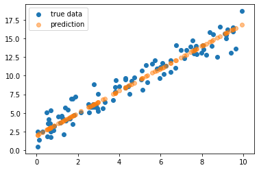
d) Apply the trained model to x and plot the predictions along with the true values in a scatter plot
print(model.linear.weight, model.linear.bias)
with torch.no_grad():
    predictions = model(x)
    plt.scatter(x, y, label = 'true data')
    plt.scatter(x, predictions, label = 'prediction', alpha = .5)
    plt.legend()
    plt.show()
Parameter containing:
tensor([[1.4959]], requires_grad=True) Parameter containing:
tensor([2.0031], requires_grad=True)