
KMeans
Published:
![]()
MindNote - Machine Learning - Unsupervised Learning - Clustering
Author: Christian M.M. Frey
E-Mail: christianmaxmike@gmail.com
K-Means
Idea of the kmeans is that given an input data, we want to find a clustering such that the within-cluster variation of each cluster is small and we use the centrois of a cluster as the representative of them. Hence, the objective for a given $k$ is to form $k$ groups such that the sum of the (squared) distances between the mean of the groups and their elements is minimal.
The objective function, we try to optimize is defined as: \(J = \sum_{i=0}^{k} \sum_{m \in C_i} (m - c_i)^2\) where $c_i$ denotes the centroid of the cluster $C_i$.
Load dependencies
%matplotlib inline
import matplotlib.pyplot as plt
import seaborn as sns;
import numpy as np
sns.set()
from sklearn.metrics import silhouette_samples, silhouette_score
import math
import matplotlib.cm as cm
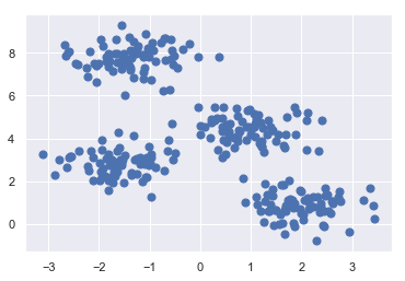
from sklearn.datasets.samples_generator import make_blobs
X, y_true = make_blobs(n_samples=300, centers=4, cluster_std=0.60, random_state=0)
plt.scatter(X[:, 0], X[:, 1], s=50);
Implementation of KMeans
class KMeans (object):
"""
Implementation of the KMeans algorithm
Arguments:
n_clusters: number of clusters
centroids: the centroids describing the cluster representatives
seed: random seed
Properties:
n_clusters: number of clusters
centroids: centroids being the cluster representatives
random_gen: random number generator (for initializing the centroids)
cls_labels: the labels of the datapoints,i.e., indicator to which cluster a point
is affiliated
"""
def __init__(self, n_clusters, centroids=None, seed=42):
self.n_clusters = n_clusters
self.centroids = centroids
self.random_gen = np.random.RandomState(seed)
self.cls_labels = None
def _euclidean (self, x, y):
"""
calculates the l2 distance between two vectors
Returns:
the l2 distance (euclidean distance)
"""
return math.sqrt(sum([(a - b) ** 2 for a, b in zip(x, y)]))
def _pick_random_centroids(self, X):
"""
method for initializing random centroids. Picks n random points out of the dataset,
where n is the number of clusters
Returns:
n number of centroids, where n is the number of clusters
"""
centroids = X[self.random_gen.choice(X.shape[0], self.n_clusters, replace=False), :]
return centroids
def _plot_clustering(self, X, it):
"""
Method for plotting the current clustering. We plot the dataset, the current
centroids and colors indicate the cluster affiliation
Arguments:
X: the dataset the algorithm is performed on
it: the current iteration number
(can be used e.g. as an additional information in the title)
"""
plt.figure()
plt.title("Iteration {d}".format(d=it))
plt.scatter(X[:, 0], X[:, 1], c=self.cls_labels, s=50, cmap='viridis');
plt.scatter(self.centroids[:, 0], self.centroids[:, 1], s=100, c='w', edgecolor="red")
plt.title("The visualization of the clustered data.")
plt.xlabel("Feature space for the 1st feature")
plt.ylabel("Feature space for the 2nd feature")
def fit(self, X, max_iteration=100):
"""
Method used for executing the KMeans algorithm.
Arguments:
X: the dataset
max_iteration: the maximal number of iterations being performed
"""
# Choose random centroids
self.centroids = self._pick_random_centroids(X)
iteration = 1
while True:
# Find closest centroid
self.cls_labels = np.array([np.argmin([self._euclidean(x, c_i) for c_i in self.centroids]) for x in X])
# calculation of silhouette score
# silhouette_avg = silhouette_score(X, self.cls_labels)
# plot clustered data
self._plot_clustering(X,iteration)
# Compute new centroids by means of points being assigned to each cluster
new_centroids = np.array([X[self.cls_labels == i].mean(axis=0) for i in range(self.n_clusters)])
# Check termination criteria
if np.all(self.centroids == new_centroids) or iteration > max_iteration:
break
# Assign new centroids
self.centroids = new_centroids
iteration += 1
def fit_silhouette(self, X, max_iteration=100):
"""
Method used for executing the KMeans algorithm. In addition it plots the silhouette coefficients.
Arguments:
X: the dataset
max_iteration: the maximal number of iterations being performed
"""
# Choose random centroids
self.centroids = self._pick_random_centroids(X)
iteration = 1
while True:
# Find closest centroid
self.cls_labels = np.array([np.argmin([self._euclidean(x, c_i) for c_i in self.centroids]) for x in X])
fig, (ax1, ax2) = plt.subplots(1, 2)
fig.set_size_inches(12, 4)
ax1.set_ylim([0, len(X) + (self.n_clusters + 1) * 10])
ax1.set_title("The silhouette plot for the various clusters.")
ax1.set_xlabel("The silhouette coefficient values")
ax1.set_ylabel("Cluster label")
silhouette_avg = silhouette_score(X, self.cls_labels)
# The vertical line for average silhouette score of all the values
ax1.axvline(x=silhouette_avg, color="red", linestyle="--")
print("For n_clusters =", self.n_clusters, "The average silhouette_score is :", silhouette_avg)
# plt.figure()
plt.title("$Iteration {d}$".format(d=iteration))
ax2.scatter(X[:, 0], X[:, 1], c=self.cls_labels, s=25, cmap='viridis');
ax2.scatter(self.centroids[:, 0], self.centroids[:, 1], s=100, c='w', edgecolor="red")
ax2.set_title("The visualization of the clustered data.")
ax2.set_xlabel("Feature space for the 1st feature")
ax2.set_ylabel("Feature space for the 2nd feature")
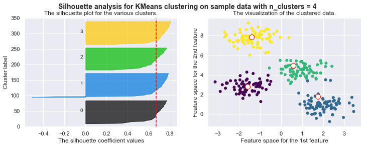
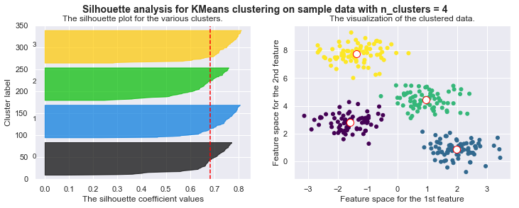
plt.suptitle(("Silhouette analysis for KMeans clustering on sample data "
"with n_clusters = %d" % self.n_clusters),
fontsize=14, fontweight='bold')
# Compute the silhouette scores for each sample
sample_silhouette_values = silhouette_samples(X, self.cls_labels)
y_lower = 10
for i in range(self.n_clusters):
# Aggregate the silhouette scores for samples belonging to
# cluster i, and sort them
ith_cluster_silhouette_values = sample_silhouette_values[self.cls_labels == i]
ith_cluster_silhouette_values.sort()
size_cluster_i = ith_cluster_silhouette_values.shape[0]
y_upper = y_lower + size_cluster_i
color = cm.nipy_spectral(float(i) / self.n_clusters)
ax1.fill_betweenx(np.arange(y_lower, y_upper),
0, ith_cluster_silhouette_values,
facecolor=color, edgecolor=color, alpha=0.7)
# Label the silhouette plots with their cluster numbers at the middle
ax1.text(-0.05, y_lower + 0.5 * size_cluster_i, str(i))
# Compute the new y_lower for next plot
y_lower = y_upper + 10 # 10 for the 0 samples
# Compute new centroids by means of points being assigned to each cluster
new_centroids = np.array([X[self.cls_labels == i].mean(axis=0) for i in range(self.n_clusters)])
# Check termination criteria
if np.all(self.centroids == new_centroids) or iteration>max_iteration:
break
# Assign new centroids
self.centroids = new_centroids
iteration += 1
Run it!
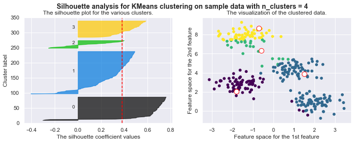
kmeans = KMeans(n_clusters=4)
kmeans.fit_silhouette(X)
For n_clusters = 4 The average silhouette_score is : 0.38145632079855524
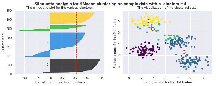
For n_clusters = 4 The average silhouette_score is : 0.4196365342575672
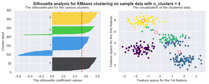
For n_clusters = 4 The average silhouette_score is : 0.5224106511612718
For n_clusters = 4 The average silhouette_score is : 0.6705159431863005
For n_clusters = 4 The average silhouette_score is : 0.6819938690643478
For n_clusters = 4 The average silhouette_score is : 0.6819938690643478

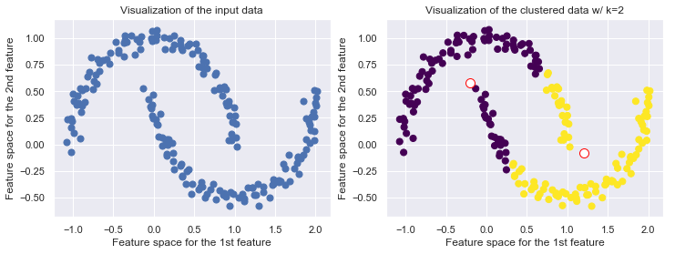
Drawbacks of KMeans
KMeans is limited to linear boundaries, i.e., clusters are forced to convex space partitions
If the data generating process has a higher complexity, i.e. if the clusters which we expect to be found have a more complicated geometry, then k-means will often be ineffective. The boundaries of clusters having been found by k-means will always be linear (think of Voronoi cell boundaries).
Recap Voronoi Diagram: For a given set of points $P = {p_1, \ldots, p_k}$, a Voronois diagram partitions the data space into so-called Voronoi cells. The cell of a point $p \in P$ covers all points in the data space for which $p$ is the nearest neighbors among the points from $P$. The Voronoi cells of two neighboring points $p_i, p_j \in P$ are separated by the perpendicular hyperplane between $p_i$ and $p_j$. Vornois cells are intersection of half spaces and thus convex regions.
from sklearn.datasets import make_moons
from sklearn.cluster import KMeans

X, y = make_moons(200, noise=.05, random_state=0)
k = 2
fig, (ax1, ax2) = plt.subplots(1,2, figsize=(12,4))
ax1.scatter(X[:, 0], X[:, 1], s=50);
ax1.set_title('Visualization of the input data')
ax1.set_xlabel('Feature space for the 1st feature')
ax1.set_ylabel('Feature space for the 2nd feature')

kmeans = KMeans(k, random_state=42)
labels = kmeans.fit_predict(X)
ax2.scatter(X[:, 0], X[:, 1], c=labels, s=50, cmap='viridis')
ax2.scatter(kmeans.cluster_centers_[:, 0], kmeans.cluster_centers_[:, 1], c='w', edgecolor='red', s=100)
ax2.set_title("Visualization of the clustered data w/ k={k}".format(k=k))
ax2.set_xlabel('Feature space for the 1st feature')
ax2.set_ylabel('Feature space for the 2nd feature')
<matplotlib.text.Text at 0x11ad24160>
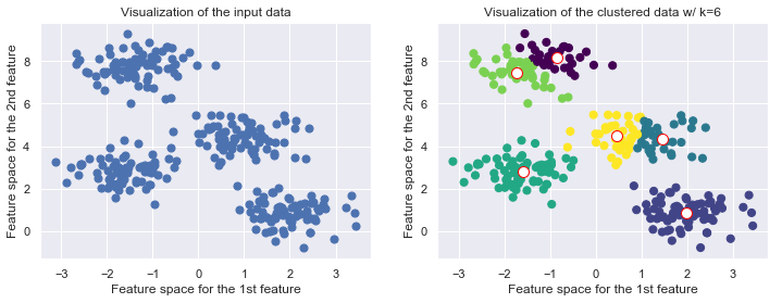
The number of clusters must be predefined
The number of clusters have to be selected beforehand by the user, i.e. k serves as a hyperparameter to tell the algorithm houw many clusters you expect to find. It cannot learn itself the number of clusters from the data.
from sklearn.datasets.samples_generator import make_blobs
from sklearn.cluster import KMeans

X, y_true = make_blobs(n_samples=300, centers=4, cluster_std=0.60, random_state=0)
k = 6

fig, (ax1, ax2) = plt.subplots(1,2, figsize=(12,4))
ax1.scatter(X[:, 0], X[:, 1], s=50);
ax1.set_title('Visualization of the input data')
ax1.set_xlabel('Feature space for the 1st feature')
ax1.set_ylabel('Feature space for the 2nd feature')

kmeans = KMeans(k, random_state=42)
labels = kmeans.fit_predict(X)
ax2.scatter(X[:, 0], X[:, 1], c=labels, s=50, cmap='viridis')
ax2.scatter(kmeans.cluster_centers_[:, 0], kmeans.cluster_centers_[:, 1], c='w', edgecolor='red', s=100)
ax2.set_title("Visualization of the clustered data w/ k={k}".format(k=k))
ax2.set_xlabel('Feature space for the 1st feature')
ax2.set_ylabel('Feature space for the 2nd feature')
<matplotlib.text.Text at 0x118e51358>
Furher drawbacks
- Applicable only when mean is defined
- Sensitive to noisy data and outliers
- Result depend on the initial partition; often terminated at a local optimum - however: methods for a good initialization exist
- kMeans can be slow for a large number of samples. Improvement can be made by approaches like batch-based-kMeans
- the KMeans algorithm is sensitive to outliers since an oject with an extremely large value may substantially distort the distribution of the data.
Additional notes:
Source for silhouette plots (scikit-learn.org): Link